Variational Inference from Scratch

Let’s derive the evidence lower bound used in variational inference using Jensen’s inequality and the Kullback-Leibler divergence.

In Bayesian inference we are often tasked with solving analytically intractable integrals. Approximate techniques such as Monte-Carlo and quadrature will work well when the variable being integrated over is low-dimensional. However, for high-dimensional integrals, practitioners often resort to Markov chain Monte-Carlo or variational inference (VI). In this article, we will cover the latter starting from the very basic primitive results encountered in high school or an undergraduate science degree.

Background

In this section we’ll briefly highlight the preliminary results required for understanding VI. The aim here is to firstly establish notation and refresh readers of certain results. If these results are unfamiliar to the reader, then an introduction to Bayesian statistics, such as the Bayesian Data Analysis book may be a more suitable starting point.

Bayes’ Theorem

The cornerstone of Bayesian statistics, Bayes’ theorem seeks to quantify the probability of an event, conditional on some observed data. The event under consideration here is arbitrary and we simply denote its value by $\theta$. We further state our prior belief about the value of $\theta$ through a prior distribution $p_{0}(\theta)$. Our observed data is denoted by $y$. Together, Bayes’ theorem can be expressed by

We'll expand more on this when we get to the topic of VI but, for completeness, we call $p(y\mid\theta)$ the likelihood and $p(y)$ the marginal likelihood.

Expectation

In $\eqref{equn:BayesTheorem}$, $\theta$ is a random variable with associated density $\pi(\theta)$. Whilst we place a prior belief $p_{0}(\theta)$ about the density of $\theta$, this, in practice, is almost certainly not the true underlying density of $\theta$. Assuming $\theta$ is a continuous random variable, the expectation operator is defined as

The expectation operator is also linear. This means that if we have a second random variable $\zeta$, then the following identity is true

Jensen’s Inequality

For a convex function $f$, Jensen’s inequality states the following inequality

Informally, a convex function $f$ is a u-shaped function such that if we pick any two values $x_1, x_2$ and draw a line between $f(x)$ and $f(y)$, then the line will be above the function's curve.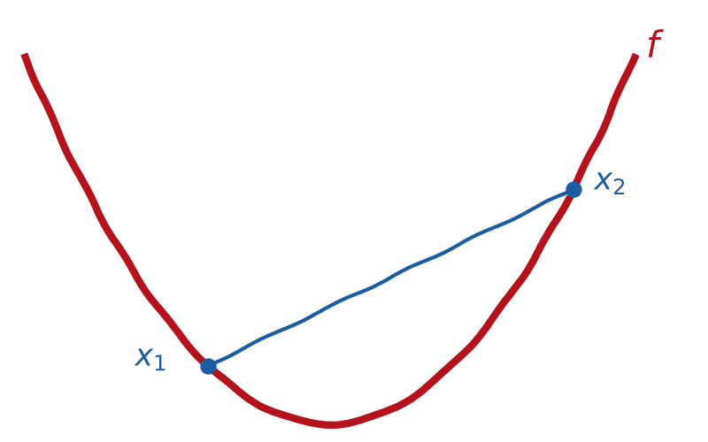 

Motivation

With the necessary mathematical in tools, I’ll now motivate the use of VI through three cases where an intractable integral can commonly occur.

Normalising Constants

Bayes’ theorem in $\eqref{equn:BayesTheorem}$ can be written as

The denominator here is simply the integral of the numerator with respect to our model parameters $\theta$ and its purpose is to ensure that the posterior distribution $p(\theta \mid y)$ is a valid probability density function. However, $\theta$ can often be a high-dimensional parameter and the integrand may have no nice analytical form. As such, evaluating the integral can consume a large portion of a Bayesian's time.

Marginalisation

If we introduce an additional parameter $z \in Z$ that we’d like to obtain a posterior distribution for, then we now have the joint posterior distribution $p(\theta, z \mid y)$. Assuming we can calculate this quantity, then often wish to marginalise $z$ from our joint posterior which requires evaluation of the integral

Again, in the absence of an analytical solution, the evaluation of this integral will be challenging for high-dimensional $Z$.

Expectations

If we have our posterior distribution $p(\theta\mid y)$, then we may wish to evaluate the expectation of a function of $\theta$ e.g.,

Examples of such cases are for the conditional mean where $f(\theta)=\theta$ and the conditional covariance $f(\theta) = \theta\theta' - \mathbb{E}[x]\mathbb{E}'[x]$.

Variational Inference

Hopefully by this point the need for techniques for evaluating high-dimensional and challenging integral is clear. In this derivation we’ll be considering the case of an intractable normalising constant which makes accessing our posterior distribution intractable. VI seeks resolve this issue by identifying the distribution $q_{\lambda}^{\star}$ from a family of distributions $\mathcal{Q}$ that best approximates the true posterior $p(\theta\mid y)$. $\lambda$ denotes the parameters of $q$ and are known as variational parameters.

Typically, $\mathcal{Q}$ is the family of multivariate Gaussian distributions, but this is by no means a requirement. We use the Kullback-Leibler (KL) divergence to quantify how well a candidate distribution $q\in\mathcal{Q}$ approximates $p(\theta\mid y)$ and we write this as

There are two things to note here, 1) the KL-divergence is asymmetric (To see this, simply rewrite $\eqref{equn:KLDiv}$ with $q$ and $p$ reversed) and 2) we have dropped the dependence of $q$ on $\lambda$ for notational brevity.

We define our optimal distribution $q^{\star}\in\mathcal{Q}$ as the distribution that satisfies

Clearly this objective is intractable as simply evaluating the KL divergence term in $\eqref{equn:OptimalQ}$ would require evaluating $p(y)$ - the very reason we have had to resort to VI in the first place. To circumvent this we introduce the evidence lower bound (ELBO). The ELBO, as the name might suggest, provides a lower bound on $\log p(y)$ that we can tractably optimise as the KL divergence is always greater than or equal to zero. When $q(\theta) = p(\theta\mid y)$, then clearly the ELBO is equal to the marginal log-likelihood.

We will now proceed to derive the ELBO in two ways: first using the definition of the KL divergence from $\eqref{equn:KLDiv}$ and secondly by applying Jensen’s inequality from $\eqref{equn:Jensens}$ to $\log p(y)$.

KL Divergence Derivation

From $\eqref{equn:KLDiv}$ we can rewrite the KL divergence in terms of expectations

By the linearity of the expectation, we now have the following

The final step relies on the face that $p_{0}(\theta)$ is independent of $q(\theta)$ and the expectation is simply a constant i.e., $\mathbb{E}q[\log p{0}(\theta)] = \log p_{0}(\theta) \mathbb{E}_q[1]$.

We now introduce the ELBO of $q$, denoted $\operatorname{ELBO}(q)$ as the following