Variational Inference by Implementation

2025-10-07

A gentle introduction to variational inference applied to Bayesian logistic regressions with accompanying PyTorch implementation.

Introduction

The most common problem that one faces in a Bayesian workflow is computing the posterior distribution. Markov chain Monte-Carlo (MCMC) offers one solution to this issues, but variational inference (VI) is an appealing alternative. In contract to MCMC, VI seeks to approximate the intractable posterior distribution by optimising the parameters of a tractable parametric variational distribution such that the distance between the variational distribution and the true posterior is minimised.

By virtue of being an optimisation-based approach, VI can offer several advantages over MCMC:

It scales naturally to large datasets using stochastic gradient methods.
It can leverage GPUs for more efficient computations.
It provides explicit control over the complexity–accuracy trade-off through the choice of variational family.

The cost of these benefits is an approximation. Unlike MCMC, there are no guarantees that VI will eventually return the true posterior. This is primarily driven by the fact that we, as the practitioner, are forced to choose the family of distributions $Q$ that our variational distribution is a member of. Oftentimes, for computational convenience, $Q$ is chosen to be the family of (multivariate) Gaussian. Therefore, unless the true posterior is itself a Gaussian, then there is little chance that our variational distribution will ever become equivalent to the true posterior.

Mathematical Details

For an observed dataset $D$ and parameters $θ$ , our posterior may be written as

p (θ ∣ D) = \frac{p (D ∣ θ) p (θ)}{p (D)} .

Letting the $Q$ , the variational family, be the set of multivariate Gaussian, we write a single variational distribution be written as

q_{λ} (θ) = N (θ ∣ μ, Σ)

where $λ$ is the variational distribution’s parameters.

To identify the optimal variational approximation $q^{⋆}$ , we seek to minimise

KL (q_{λ} (θ) ∣∣ p (θ ∣ D)),

to yield the objective

q^{⋆} = \arg min_{q \in Q} KL (q_{λ} (θ) ∣∣ p (θ ∣ D)) .

where $KL$ denotes the Kullback-Leibler divergence (KLD).

Unfortunately, computing the KLD from the variational distribution to the true posterior is intractable. We are, therefore, required to reformulate the objective into a lower bound by rearranging, expanding, and bounding via Jensen’s inequality. A full derivation is given in Variational Inference from Scratch. The bound is known as the evidence lower bound (ELBO), and we write it as

ELBO = E_{q} [\log p (D ∣ θ)] - KL (q_{λ} (θ) ∣∣ p (θ)) .

The ELBO consists of two terms. The first, the expected log-likelihood, encourages the variational distribution to explain the observed data. The second term is the Kullback-Leibler divergence between the variational distribution and the prior, which acts as a regulariser. Our objective is to maximise the ELBO with respect to the variational parameters $λ$ .

We shall now proceed to implement this routine.

 1
 2
 3
 4
 5
 6
 7
 8
 9
10
11
import math
import torch
from torch import nn
import torch.nn.functional as F
import matplotlib.pyplot as plt
from tqdm.auto import trange
from sklearn.datasets import make_moons

SEED = 123
torch.manual_seed(SEED)
device = torch.device("cuda" if torch.cuda.is_available() else "cpu")

Show plotting code

 1
 2
 3
 4
 5
 6
 7
 8
 9
10
11
12
13
14
15
16
17
18
19
20
21
22
23
24
25
26
27
28
29
30
31
32
33
34
35
36
37
38
39
40
41
42
43
44
45
46
47
48
49
50
51
52
53
54
55
56
57
58
59
60
61
62
63
64
65
66
67
68
69
70
71
72
73
74
75
76
77
78
79
80
81
82
83
84
85
86
87
88
89
90
91
92
93
94
95
96
97
98
99
import matplotlib.pyplot as plt
import torch


def build_mesh(
    inputs: torch.Tensor, /, grid_size: int = 150, boundary_buffer: float = 0.5
) -> tuple[torch.Tensor, torch.Tensor, torch.Tensor]:
    x1_min, x1_max = (
        inputs[:, 0].min().cpu() - boundary_buffer,
        inputs[:, 0].max().cpu() + boundary_buffer,
    )
    x2_min, x2_max = (
        inputs[:, 1].min().cpu() - boundary_buffer,
        inputs[:, 1].max().cpu() + boundary_buffer,
    )
    x1_grid = torch.linspace(x1_min, x1_max, grid_size)
    x2_grid = torch.linspace(x2_min, x2_max, grid_size)
    X1_mesh, X2_mesh = torch.meshgrid(x1_grid, x2_grid, indexing="ij")

    grid = torch.stack([X1_mesh.flatten(), X2_mesh.flatten()], dim=1)
    return grid, X1_mesh, X2_mesh


def plot_predictions(
    inputs: torch.Tensor,
    outputs: torch.Tensor,
    mean_prob: torch.Tensor,
    stddev_prob: torch.Tensor,
):
    _, X1_mesh, X2_mesh = build_mesh(inputs)

    fig, axes = plt.subplots(1, 2, figsize=(14, 5.5))

    ax1 = axes[0]
    contour1 = ax1.contourf(
        X1_mesh.cpu(), X2_mesh.cpu(), mean_prob, levels=20, cmap="RdYlBu_r", alpha=0.8
    )
    ax1.contour(
        X1_mesh.cpu(),
        X2_mesh.cpu(),
        mean_prob,
        levels=[0.5],
        colors="black",
        linewidths=2,
    )
    ax1.scatter(
        inputs[outputs == 0, 0].cpu(),
        inputs[outputs == 0, 1].cpu(),
        s=25,
        c="blue",
        edgecolors="darkblue",
        alpha=0.7,
        label="Class 0",
    )
    ax1.scatter(
        inputs[outputs == 1, 0].cpu(),
        inputs[outputs == 1, 1].cpu(),
        s=25,
        c="red",
        edgecolors="darkred",
        alpha=0.7,
        label="Class 1",
    )
    plt.colorbar(contour1, ax=ax1, label="P(y=1|x)")
    ax1.set_title("Mean Predictive Probability", fontsize=12, fontweight="bold")
    ax1.set_xlabel("x₁", fontsize=11)
    ax1.set_ylabel("x₂", fontsize=11)
    ax1.legend(fontsize=9)
    ax1.grid(alpha=0.2)

    # Right: Predictive uncertainty
    ax2 = axes[1]
    contour2 = ax2.contourf(
        X1_mesh.cpu(), X2_mesh.cpu(), stddev_prob, levels=20, cmap="viridis", alpha=0.85
    )
    ax2.scatter(
        inputs[outputs == 0, 0].cpu(),
        inputs[outputs == 0, 1].cpu(),
        s=25,
        c="lightblue",
        edgecolors="darkblue",
        alpha=0.6,
    )
    ax2.scatter(
        inputs[outputs == 1, 0].cpu(),
        inputs[outputs == 1, 1].cpu(),
        s=25,
        c="lightcoral",
        edgecolors="darkred",
        alpha=0.6,
    )
    plt.colorbar(contour2, ax=ax2, label="Std(p)")
    ax2.set_title("Predictive Uncertainty (Epistemic)", fontsize=12, fontweight="bold")
    ax2.set_xlabel("x₁", fontsize=11)
    ax2.set_ylabel("x₂", fontsize=11)
    ax2.grid(alpha=0.2)

    plt.tight_layout()
    plt.show()

Implementation

Goal

Our goal in this notebook is to use VI to approximate the posterior of a Bayesian logistic regression model.

Core Structures

In the first stage of our implementation, we shall define the core components for our VI algorithm. This includes the variational distribution itself, a function to compute the KL divergence to the prior, and a function to compute the ELBO, our objective function.

The following code defines:

MeanFieldGaussian: A class for our mean-field variational distribution. It uses the reparameterisation trick for sampling and a softplus transformation to ensure positive standard deviations.
gaussian_kl_meanfield: A function for the analytical computation of the KL divergence between our variational distribution and the Gaussian prior.
elbo_logistic_regression: A function that computes a Monte Carlo estimate of the ELBO. It combines the expected log-likelihood of the data with the KL divergence term.

 1
 2
 3
 4
 5
 6
 7
 8
 9
10
11
12
13
14
15
16
17
18
19
20
21
22
23
24
25
26
27
28
29
30
31
32
33
34
35
36
37
38
39
40
41
42
43
44
45
46
47
48
49
50
51
52
53
54
55
56
57
58
59
60
61
62
JITTER = 1e-6


class MeanFieldGaussian(nn.Module):
    """Mean-field Gaussian variational distribution. The standard deviation is
    parameterized as σ = softplus(ρ) + jitter to ensure positivity and numerical stability.
    """

    def __init__(self, num_dims: int, rho: float = -1.0):
        super().__init__()
        self.location = nn.Parameter(torch.zeros(num_dims))
        self.rho = nn.Parameter(torch.full((num_dims,), rho))

    @property
    def stddev(self):
        return F.softplus(self.rho) + JITTER

    def sample(self, num_samples: int = 1):
        """Sample from the variational distribution using the reparameterization trick."""
        eps = torch.randn(
            num_samples, self.location.numel(), device=self.location.device
        )
        return self.location + self.stddev * eps


def gaussian_kl_meanfield(
    location: torch.Tensor, stddev: torch.Tensor, prior_stddev: torch.Tensor
):
    """Compute KL divergence KL[q(w) || p(w)] for diagonal Gaussian distributions."""
    variance = stddev**2
    prior_variance = prior_stddev**2
    return 0.5 * torch.sum(
        (variance + location**2) / prior_variance
        - 1.0
        + 2.0 * torch.log(prior_stddev / stddev)
    )


def elbo_logistic_regression(
    variational_dist: MeanFieldGaussian,
    inputs: torch.Tensor,
    outputs: torch.Tensor,
    prior_stddev: torch.Tensor,
    /,
    num_samples: int = 20,
):
    """Compute the Evidence Lower Bound (ELBO) for Bayesian logistic regression.

    ELBO = 𝔼_q[log p(y|X,w)] - KL[q(w) || p(w)]
    """
    weight_samples = variational_dist.sample(num_samples)
    bias_term = torch.ones(inputs.shape[0], 1, device=inputs.device)
    augmented_inputs = torch.cat([bias_term, inputs], dim=1)
    logits = augmented_inputs @ weight_samples.transpose(0, 1)
    log_lik = -F.binary_cross_entropy_with_logits(
        logits, outputs.unsqueeze(1).expand_as(logits), reduction="none"
    )
    expected_log_likelihood = log_lik.mean(dim=1).sum()
    kl_term = gaussian_kl_meanfield(
        variational_dist.location, variational_dist.stddev, prior_stddev
    )
    return expected_log_likelihood - kl_term

Data Prep

To test our implementation, we will use a synthetic dataset generated by the make_moons function from scikit-learn. To enable our logistic regression model to learn the non-linear decision boundary, we will augment the original 2D features with polynomial terms (e.g., $x_{1}^{2}, x_{2}^{2}, x_{1} x_{2}$ ). This transformation maps the data into a higher-dimensional space where a linear separation for the moons data becomes possible.

 1
 2
 3
 4
 5
 6
 7
 8
 9
10
11
12
13
14
15
def polynomial_features(inputs: torch.Tensor):
    """Transform 2D inputs into polynomial feature space."""
    x1, x2 = inputs[:, 0:1], inputs[:, 1:2]
    return torch.cat([x1, x2, x1**2, x2**2, x1 * x2], dim=1)


num_data = 300
prior_stddev = 1.0

raw_inputs, outputs = [
    torch.from_numpy(_x).float()
    for _x in make_moons(n_samples=num_data, noise=0.2, random_state=SEED)
]

inputs = polynomial_features(raw_inputs)

Training

Now we are ready to train our model. The training process involves optimising the parameters of the variational distribution—its mean and standard deviation—to maximise the ELBO.

We use the Adam optimiser for this task. In each iteration of the training loop, we iterate the following steps:

Calculate a stochastic estimate of the ELBO using a number of samples from the variational distribution.
Compute the gradients of the negative ELBO with respect to the variational parameters. We use the negative ELBO because optimisers in PyTorch perform minimisation.
Perform a gradient-step update of the variational parameters.

 1
 2
 3
 4
 5
 6
 7
 8
 9
10
11
12
13
14
15
16
17
18
19
20
21
22
23
24
NUM_VI_SAMPLES = 50
NUM_ITERATIONS = 2000
LEARNING_RATE = 0.05

num_params = inputs.shape[1] + 1
variational_dist = MeanFieldGaussian(num_params)
opt = torch.optim.Adam(variational_dist.parameters(), lr=LEARNING_RATE)

pbar = trange(NUM_ITERATIONS)

for t in pbar:
    opt.zero_grad()

    loss = -elbo_logistic_regression(
        variational_dist,
        inputs,
        outputs,
        torch.tensor(prior_stddev, device=device),
        num_samples=NUM_VI_SAMPLES,
    )
    loss.backward()
    opt.step()
    if (t + 1) % 500 == 0:
        pbar.set_postfix({"elbo": -loss.item()})

Visualising Predictions

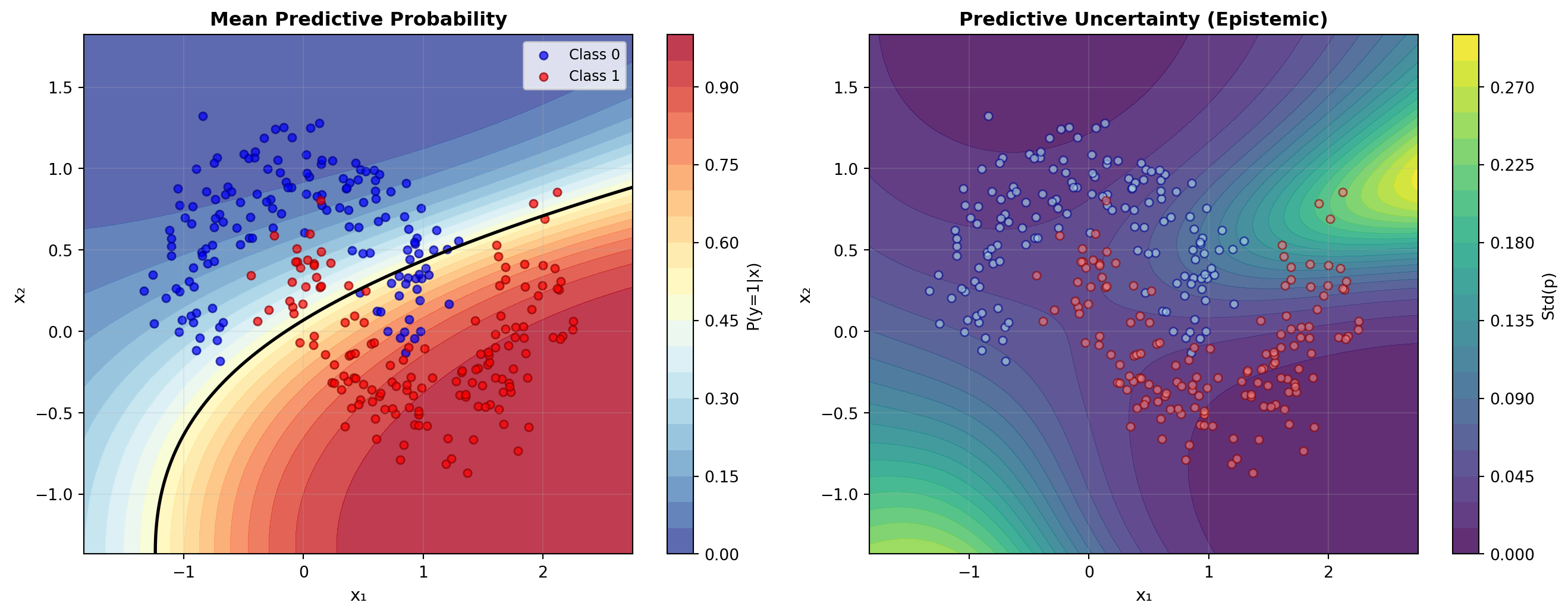
After training, our variational_dist provides an approximation to the posterior distribution over the model’s parameters. A key advantage of the Bayesian approach is the ability to quantify uncertainty, and we can now use this posterior approximation to make predictions that capture this.

To do this, we create a grid of points across the input space. For each point, we draw multiple samples of the parameters from our trained variational distribution. Each parameter sample defines a different logistic regression model and, therefore, gives a different prediction. The distribution of these predictions for a single point tells us about the model’s uncertainty at that location.

The final plot visualises both the model’s predictions and its uncertainty. We show the mean predictive probability, which is the average of the predictions across all parameter samples and represents the model’s effective decision boundary. Alongside this, we show the predictive uncertainty, calculated as the standard deviation of the predictions. This standard deviation is a measure of epistemic uncertainty—uncertainty in the model’s parameters—and we expect it to be higher in regions with little data.

 1
 2
 3
 4
 5
 6
 7
 8
 9
10
11
12
13
14
15
16
17
18
19
NUM_PRED_SAMPLES = 200
GRID_SIZE = 150
PLOT_BUFFER = 0.5

grid, _, _ = build_mesh(raw_inputs)
input_grid = polynomial_features(grid).to(device)


with torch.no_grad():
    weight_samples = variational_dist.sample(num_samples=NUM_PRED_SAMPLES)
    X_grid_aug = torch.cat(
        [torch.ones(input_grid.shape[0], 1, device=device), input_grid], dim=1
    )
    logits_grid = X_grid_aug @ weight_samples.transpose(0, 1)
    probs_grid = torch.sigmoid(logits_grid)
    mean_prob = probs_grid.mean(dim=1).cpu().reshape(GRID_SIZE, GRID_SIZE)
    stddev_prob = probs_grid.std(dim=1).cpu().reshape(GRID_SIZE, GRID_SIZE)

plot_predictions(raw_inputs, outputs, mean_prob, stddev_prob)